Data Management

View and Discover Available Data

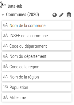
The data panel shows the available datasets list for the actual map (queries of the actual map and imported files).

It is possible to rename the data sets using the edit mode, by clicking on the pencil button when hovering with the mouse over the Data panel. After clicking on the edit button the data set will be opened in edit mode. The padlock icon indicates that the data set is private, i.e. it is visible only by you.

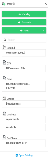
Each dataset can be unfolded and layers can be added to the map using a single drag and drop:

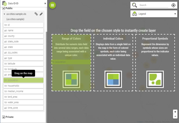
The rights can vary according to the dataset. When a user is not allowed to edit a dataset, then creation of layers by drag and drop is forbidden.

Adding Data

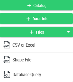
The intermediate users and above add data using the buttons:

Type	Description
Data Hub	The Data Hub provides a turnkey dataset
CSV / Excel	Addition of a CSV/Excel file
Shapefile	Addition of a shapefile
Catalog	Addition of common data to the organization from the catalog. The catalog is accessible from the Administration.
Database Query	This feature allows to define a data set from an SQL query (requires the "configSQL" role. See section 9.9 SQL Query.

CSV/Excel import is available through an extension and the functionality is controlled by the product license.

The catalog represents the list of vector map services declared in the administration console. Also included are territory management projects that have been published.

The table below summarizes all the possibilities regarding the rights:

User Type	Dataset Privacy	Owner?	Can view?	Is editable?
End User	Public	Cannot import	YES	NO
End User	Private	Cannot import	NO	NO
Intermediary User	Private	YES	YES	YES
Intermediary User	Private	NO	NO	YES
Intermediary User	Public	NO	YES	NO
Author/Designer	Public	YES	YES	YES
Author/Designer	Public	NO	YES	YES
Author/Designer	Private	YES	YES	YES
Author/Designer	Private	NO	NO	NO

As soon as the data is imported, the Data Editor opens.

The Data Editor can be opened any time one clicks on the button.

Data-Hub

The Data-Hub provides direct access to a whole set of socio-economic data directly from the Galigeo map.

The access is by clicking on the + button on the Data panel.

The main window of the Data-Hub has the different available indicators sorted by geographical levels.

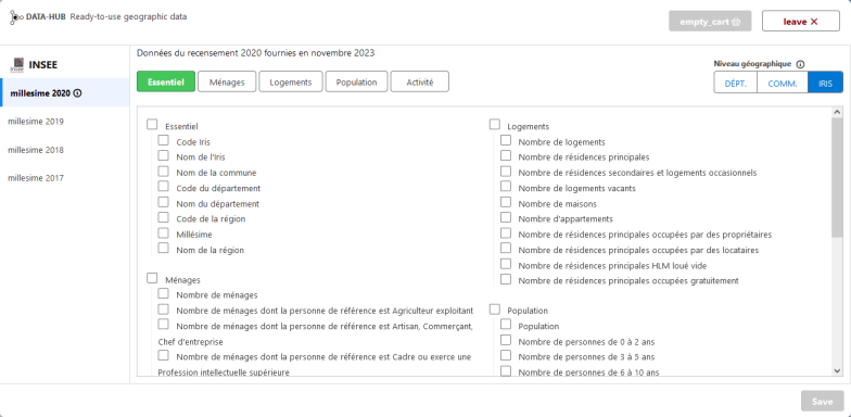
Once the indicators chosen, after saving the selection, a new dataset will appear in the Data panel.

The indicators list can be updated any time by using the button.

Layers from the Data-Hub automatically appear in the list of geographic layers used to make a join. When a join is based on a Data-Hub layer, the indicators from Data-Hub are automatically added to the dataset.

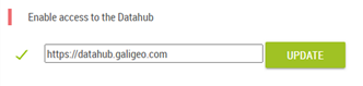
If the Data-Hub icon is not present, it can be activated from the Administration index page (Galigeo Cloud not concerned). This action requires an administrator profile.

For on premise versions, the Galigeo server must be able to access the Internet.

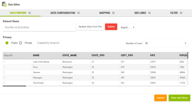
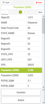
Data Preview

The data preview displays a subset of the current dataset. The panel allows to:

• Rename the dataset
• Delete the dataset
• Update the dataset (this is used to update the data, however make sure to re-import a file that has exactly the same structure). This button is not available at the initial import of the dataset.
• Export the dataset as CSV, GeoJson or Shape file or to the catalog
• Make the dataset private/public

Depending of the dataset type, some of these controls can be missing. For example, catalog dataset cannot be re-imported since it is linked to an existing catalog layer. In some cases, a user might not be authorized to edit the dataset; in which case most controls are disabled.

The file used for update has to have exactly the same structure (number and names of columns) and has to be the same type as the original file used when the dataset was imported.

Geocoding

It is possible to ask for an automatic geocoding using this button :

This is dependent of how many geocoding credits you have available. Using this functionality it is possible to geocode a file automatically.

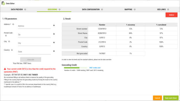
When clicking on this button, a new tab "GEOCODING" opens:

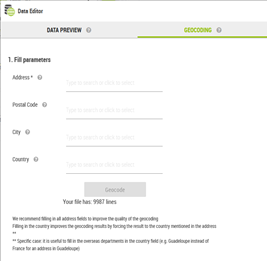
The following fields are to be filled in:

• Address
• Postal Code
• City
• Country

In order to perform a geocoding, it is mandatory to fill in the first field "Address", and it can be composed of a house number and/or a street name (e.g. 87 avenue d'Italie). Otherwise the "Geocode" button does not activate.

The other fields are optional, however we would suggest to enter all the fields in order to improve the geocoding quality.

Also, it is useful to enter the name of the country, and this will improve the geocoding results by forcing the results to comply to the country mentioned in the address. You can either enter the country or select from the drop-down list. Please note, there are specific cases of administratively speaking territories. For instance it is useful to enter the French overseas departments in the country field (e.g. Guadeloupe instead of France for a Guadeloupe address).

There is an interactive example at the bottom left corner of the screen helping with the visualisation of the address from your file.

You get also an indication about how many lines are in your file, and also how much will cost (in credits) in order to perform the geocoding operation.

For information, two types of geocoder are configurable in the administration: Galigeo, "World Wide" (Here), paid service, or "France" (Datagouv), free. In the second case there is no credits window present.

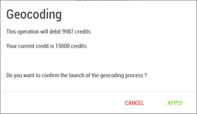
Once all the fields are filled in, you can click on the "Geocode" button, and this will open another window that will inform you how much the geocoding will cost, and how many credits will remain available.

You will have then to confirm, or not, in order to launch, or not, the geocoding.

If the number of credits is insufficient, the "Geocode" button would not activate.

The geocoding calculation is then indicated by a progress bar. You can also choose during this time to cancel the geocoding. The credits will return back to the original number. You have to pay attention though, because the geocoding might be very fast!

Once the geocoding calculation is done, the results will display as a table on the screen:

You have the choice to delete the geocoding using the button in order to perform another one on the same data set. This will again consume credits.

Data Configuration

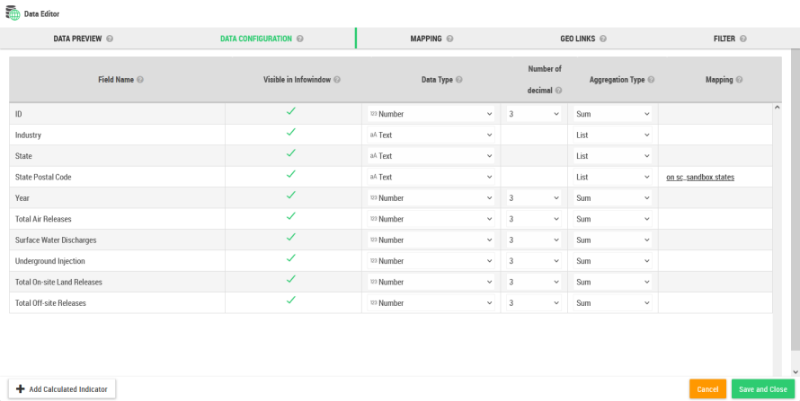
The data configuration is used to set the attributes of each individual columns. In that panel, you can:

• Rename a column
• Make it visible or not in the infowindow
• Force the data type

Some data sources have a native support for data types (Data bases, ArcGIS Server, Excel). In that case, the date dimensions are automatically recognized as date. For the other formats, Galigeo tries to recognize the date format using some common patterns.

• Define the maximal number of decimals that will be displayed (on labels, info-windows, popups, legend)
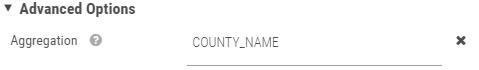
• Set the aggregation operator. This operator is applied anytime the map needs to aggregate the data.

For example an indicator can be defined by zipcode and by year in the original dataset. In that case, the indicator will be displayed by zipcode on the map and the indicators will be aggregated by year.

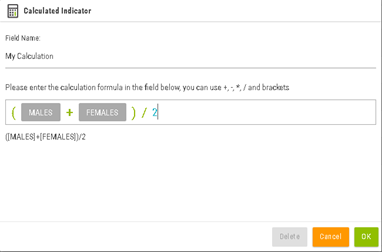
• Add a calculated indicator a combination of existing indicators.

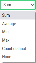
List of aggregation operators:

The following aggregation operators are available:

Operator	Description
None	Takes the first not-null value
Sum	Sum of non-null values
Average	Average of non-null values
Min	The smallest value
Max	The greatest value
Count distinct	Distinct values list from the data set

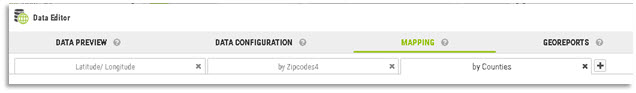
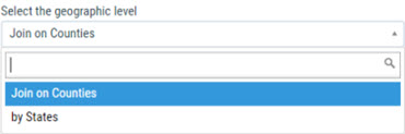
Mapping

The mapping tab is used to define how the current dataset is transformed into a geographic dataset.

The product supports three main types of mapping:

• Join on a geographic layer
• XY coordinates
• Native geometry (when the original dataset is already spatial, ex: catalog dataset)

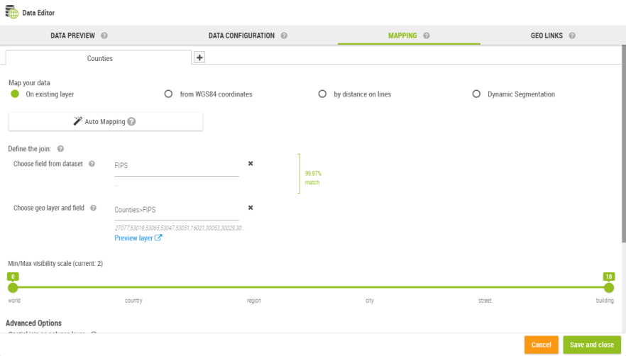
Join on a Geographic Layer

This type of mapping is a join between two datasets:

• The dataset being edited
• A geographic layer which is technically another dataset with a geometry column

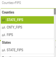
The user must select a valid join key on both sides in order to get the mapping to work.

Example: the zipcode column of a CSV with the zipcode column of a catalog layer.

The list of catalog layers displays all known geographic layers used in the application.

Finding the correct match can be difficult especially when the user is not familiar with the notion of geographic layer. To simplify the task, Galigeo provides an auto-mapping feature to automatize the process:

In most cases, this feature will find automatically the best possible mapping.

XY Coordinates

The XY mapping type is used when the dataset contains natively some X/Y columns representing the longitude/latitude coordinates of points. The XY values must be specified, as well as the used projection.

Example: The dataset represents a list of stores with two columns longitude and latitude. These columns contain the GPS coordinate of each store in degrees.

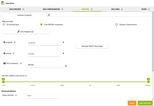
Optionally, a unique Id can be specified with this type of mapping:

The map manages automatically the data at the level of that identifier based on the aggregation operators specified.

The list of by default suggested projections can be updated by editing the file $GALIGEO_HOME/config/crs.json. The file is in this format:

json [ {"label": "WGS84", "wkid": "4326"}, {"label": "Web Mercator Auxiliary Sphere", "wkid": "3857"}, {"label": "Lambert 93", "wkid": "2154"}, {"label": "Swiss CH1903", "wkid": "1903"} ]

Where label is the display name and wkid represents the "Well Known ID" of the projection.

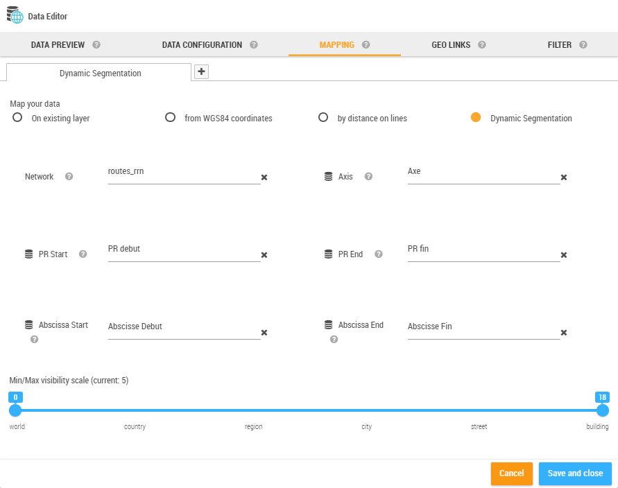
Dynamic Segmentation

The dynamic segmentation mapping is available in the form of an optional module.

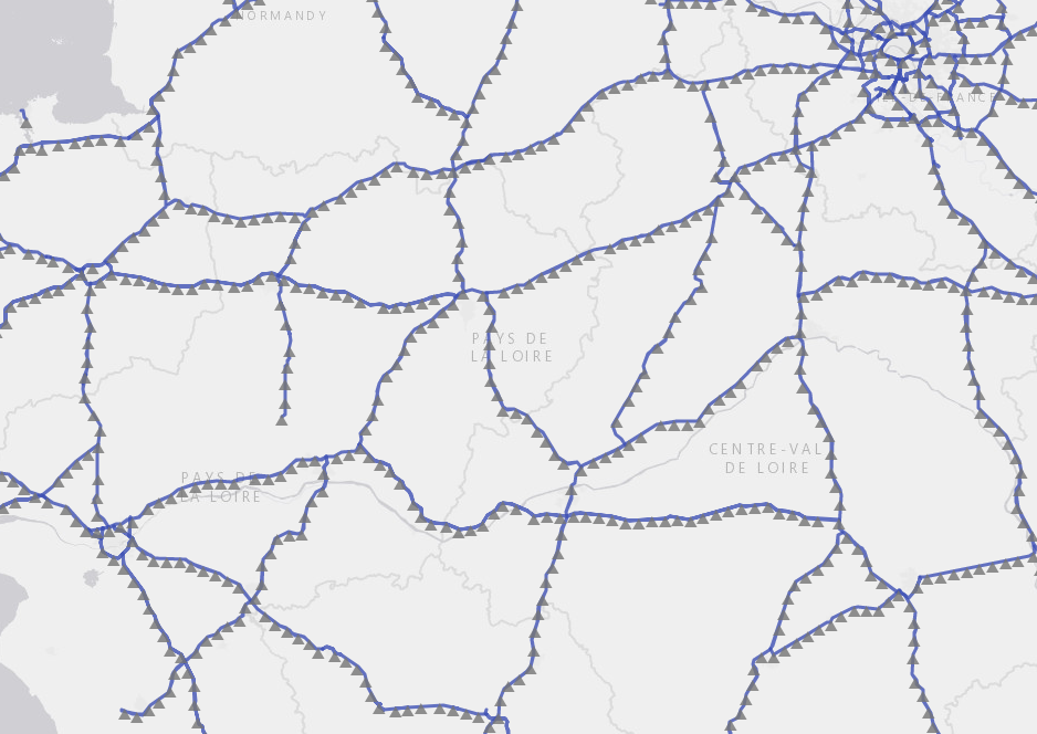
The dynamic segmentation is based on a linear data network (networks of roads, railroads, pipes, etc.) and allows the representation of segments placed between two reference points.

This implies that we have a reference points system associated to a network. For instance the milestones on roads. The available networks list is defined on the Administration.

The represented data on the map are expressed in the form PR + Abscissa, i.e. a point on the map is identified by a reference point and by a distance in meters.

Example: 50PR49D + 650 correspond to the point placed at 650 meters from the milestone 50PR49D.

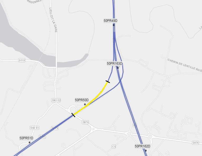
On the above example, the data received by Galigeo are expressed in the following manner:

Axis	Start PR	Start Abscissa	End PR	End Abscissa	Other Indicators ...
A86	50PR49D	650	50PR50D	200

We find the same parameters on the configuration interface of the MAPPING tab:

The Auto Mapping is not available for this type of mapping.

Network Management

The management of available networks is done from the Administration > Dynamic Segmentation.

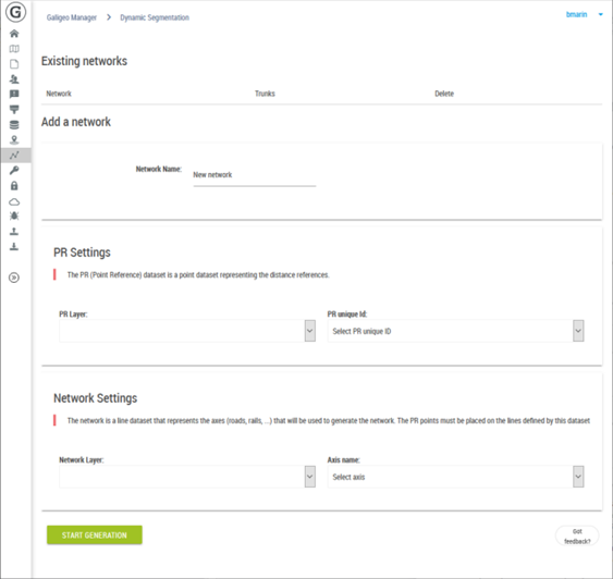
At the top of the page are listed the existent networks and allows the deleting of them if needed.

The sections "PR Settings" and "Network Settings" allow the selecting of data to use for the generation of a new network.

For the reference point one has to select from the catalog a points layer as well as the attribute that will serve to name the PRs.

For the lines, one has to select the layer representing the associated axes associated to each PR.

It is important that the two selected layers are in a relationship one to the other in order to give the expected result.

The "Start Generation" button starts the creation of the network. This operation may take several minutes according to the data to process. For this reason Galigeo is blocking the parallel creation of two networks (even from two simultaneous users).

Common Options for All Mapping Types

Auto-mapping

The auto-mapping feature is available for all mapping types.

The auto-mapping uses a smart algorithm to detect automatically how to represent a dataset on the map. In most cases, the auto-mapping is able to find itself the best representation.

It is possible the auto-mapping fails and here are the main reasons for it:

1. The catalog does not have an appropriate layer to represent the dataset. If that's the case, you need to register a new layer to the catalog (this is done once for all users).
2. The data types are not correct. For example a zipcode column might be defined as a number but is defined as a string in the geographic layer. In that case, you need to change the data type in the data configuration tab.

The auto-mapping will never select a projection layer automatically. The user always needs to specify that option manually.

Visibility Slider

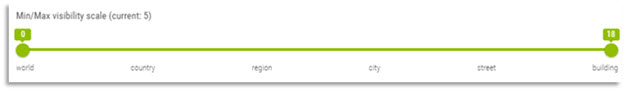
The visibility slider allows to select the visibility range of the current mapping.

Example: Let's say our data is represented at two levels: a layer US States and a layer US Counties. US States can be visible from world to country and US Counties from country to building. This way, when the map is unzoomed to the whole country, the states are visible and zooming on a state will show the counties.

Projection on layer

The current mapping can be projected on a geographic layer.

For example, let's say we have a dataset with some stores in the US represented as points on the map. The dataset can be projected on the US States layer and the result is a polygon layer representing the states and where each indicator comes from the stores but aggregated for each state.

This allows to quickly define a spatial hierarchy with the data.

Multi-Mapping

The multi-mapping is also defined from the mapping tab.

The multi-mapping is a powerful feature though it might be difficult to understand. In few words, it allows to define multiple representation types (mappers) on the same dataset.

Let's illustrate with an example: The dataset is a list of stores, each record contains the X/Y coordinates of the stores, a set of indicators (revenue, etc.) and the attached warehouse name. From that dataset, we can define 3 mappers:

• The individual stores as X/Y points
• The individual warehouse using a join on layer (the stores indicators will be aggregated for each warehouse)
• The stores by region (the result is a layer of regions where we can represent the total revenue of the stores by region)

In this example, starting from a single dataset, we quickly get a rich map showing layers on the individual stores, their attached warehouse location and the repartition through the regions.

Once various mappings are defined on a dataset, the Layer Wizard will propose the list of available mappings:

Geo-Links

The geo-links allow the association of customized links to a geographical dataset in order to query a report, an external application, or to launch a processing from a geographical selection on the map.

The geo-links are accessible complementary to the standard georeports from the info view, from a selection or in the territory management extension.

Custom URL

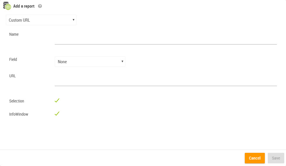
The creation of a geo-link requires 5 pieces of information:

• The georeport that was declared on the settings page
• Name: this is the name that will be displayed on the link
• Field: the field of the geographical layer which values are sent to the geo-link URL
• URL: a URL that can contain the element [values]. At runtime, [values] is replaced by the value of the "field" for the selected object. If several objects are selected, then [values] becomes a list of values separated by comma.
• Selection and/or the InfoWindow: allows the choosing of where the geolink will appear

You have the possibility to pass any values from any column of your dataset into your custom URL.

In order to do that, you need to include the column name this way in the URL: [column_name].

For instance, if you have a dataset containing 3 columns, each named column1, column2, and column3, you can pass the values of each column this way:

https://myserver.com?parameter1=[column1]&parameter2=[column2]&parameter3=[column3]

The keyword [values] is reserved by Galigeo. If you have a column named this way, its values won't be passed into the URL. Please rename your column in this case.

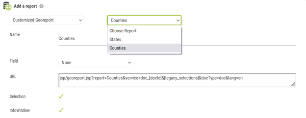
Customized Georeport

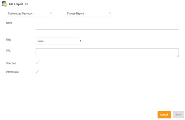
The same way, the geo links allow the calling of Excel reports. For more detail on the creation of an Excel report, see the section 9.10.1 Report Definition.

When for a map there are one or more Excel reports, it is possible to configure this report in the form of a geo link:

1. Select Customized Georeport
2. Choose the report to use from the drop-down list that appears. The fields of the Georeport fill in automatically.
3. In the list "Field", select the join field which will feed the report

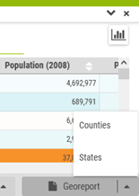
The Access Methods to Georeports

The georeports are accessible in 4 different ways:

1. Directly from the reports panel (the report is called without any geographical selection)

1. From the info-window by clicking on an object on the map

1. Using the selection tool when a selection is active

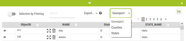
1. From a territory layer

Filters

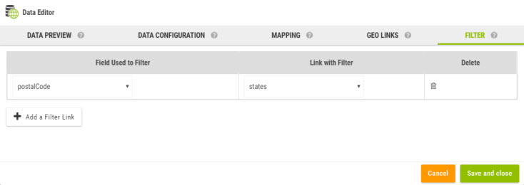
When a map contains one or several filters, it is possible to apply a filter on a layer added and known uniquely by the viewer. This regards the layers resulted from spatial queries or from imported files in the viewer, as well as GIS layers as Webservices.

This implies to have a common attribute with identical values between the filters and the geographical layer to be filtered.

In order to attach a filter to a dataset, one has to go to the tab FILTER from the Data Editor and enter two values:

• The name of the dataset field that will serve as filter
• The name of the filter to use of which the selected values will serve the filtering